Chapter 4: Vestries, justices and their opponents: 1731–1748

link to chapter 4

Packages

library(readxl)
library(janitor)
library(lubridate)
library(scales)
library(patchwork)
library(tidyverse)


# ggplot_extras ####

theme_set(theme_minimal()) # set preferred ggplot theme 
theme_update(plot.title = element_text(size = rel(1.1), hjust = 0)) # adjustments to theme
update_geom_defaults("line", list(size = 0.85)) 

Offences Prosecuted

The trend line in the original graph was recreated by using ggplot’s geom_smooth() with the method “gam” (generalized additive model).

c4_ob <-
  read_xlsx("datasets/Crime_Prosecutions.xlsx", sheet = "Old Bailey", skip = 2) %>%
  clean_names(case="lower_camel")

c4_ob_long <-
  c4_ob %>%
  filter(between(year, 1725, 1750)) %>%
  select(year, totalOffences, theftAndViolentTheft, allOtherOffences = excludingTheftAndViolentTheft) %>%
  gather("k", "v",totalOffences:allOtherOffences)  %>%
  mutate(z = case_when(
    k=="totalOffences" & year <=1747 ~ v,
    TRUE ~ NA_real_
  ))


c4_fig1_brk <- c("totalOffences", "theftAndViolentTheft", "allOtherOffences", "Trend")

c4_fig1_lab <- c("Total", "Theft and\nviolent theft", "All other\ncrime categories", "Trend line\n(1725-47)")

c4_ob_long_ggplot <-
c4_ob_long  %>%
  ggplot(aes(x=year  )) +
  geom_line(aes(y=v, colour=k, group=k, linetype=k)) +
  geom_smooth(aes(y=z, colour="Trend", linetype="Trend"), se=FALSE, method="gam", na.rm = TRUE) +
  scale_colour_manual(values=c("#0072B2", "#E69F00", "#D55E00", "#0072B2"), 
                      breaks=c4_fig1_brk, labels=c4_fig1_lab) +
  scale_linetype_manual(values = c("solid", "solid", "solid", "dotted"), 
                        breaks=c4_fig1_brk, labels=c4_fig1_lab) +
  scale_y_continuous(breaks = seq(0,750, 150)) +
  scale_x_continuous(breaks = seq(1725, 1750, 2)) +
  guides(colour=guide_legend(title=NULL), linetype=guide_legend(title=NULL)) +
  theme(legend.key.height = unit(1.7, "line") ) +
  labs(x="year", y="offences", title="Figure 4.1: Offences prosecuted at the Old Bailey, 1725–1750")

c4_ob_long_ggplot

## `geom_smooth()` using formula 'y ~ s(x, bs = "cs")'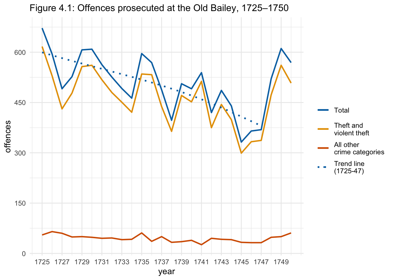

Figure 4.1: Offences prosecuted at the Old Bailey, 1725–1750

Online dataset: Crime Prosecutions (xlsx)

Workhouse Admissions

# I think the "New names" message is generated because the sheet has some random text in cells outside the main data range, which are treated as columns without headings 

c4_smwhr <-
  read_xlsx("datasets/St_Martins_Workhouse_Registers.xlsx", sheet = "St Martins Workhouse 1731-1748", skip = 26) %>%
  clean_names(case="lower_camel") %>%
  filter(age !="Totals")

## New names:
## * `` -> ...6
## * `` -> ...7
## * `` -> ...8
## * `` -> ...9
## * `` -> ...10
## * ...

c4_smwhr_long <-
  c4_smwhr %>%
  select(age, women, men, unknown) %>%
  gather("k", "v",women:unknown) %>%
  # take out unknown
  filter(k !="unknown") %>%
  # rename age labels; make them more concise
  mutate(age = fct_recode(age, `<1 year`= "0 to twelve months", `80+`="80 and over")) %>%
  mutate(age = str_replace(age, " to ", "-")) %>%
  # fix order in legend
  mutate(age = fct_relevel(age, "5-9", after = 2L)) %>%
  mutate(k = fct_recode(k, Male="men", Female="women"))


c4_smwhr_long_ggplot <-
c4_smwhr_long  %>%
  ggplot(aes(x=age, y=v, colour=k, group=k )) +
  geom_line() +
  scale_y_continuous(breaks = seq(0,900, 150)) +
  scale_colour_manual(values = c("#D55E00", "#0072B2"), breaks=c("Female", "Male")) +
  guides(colour=guide_legend(title=NULL)) +
  theme(axis.text.x = element_text(angle=90)) +
  labs(x="age group", y="admissions", title = "Figure 4.2:  St Martin in the Fields workhouse admissions, 1738-1748")

c4_smwhr_long_ggplot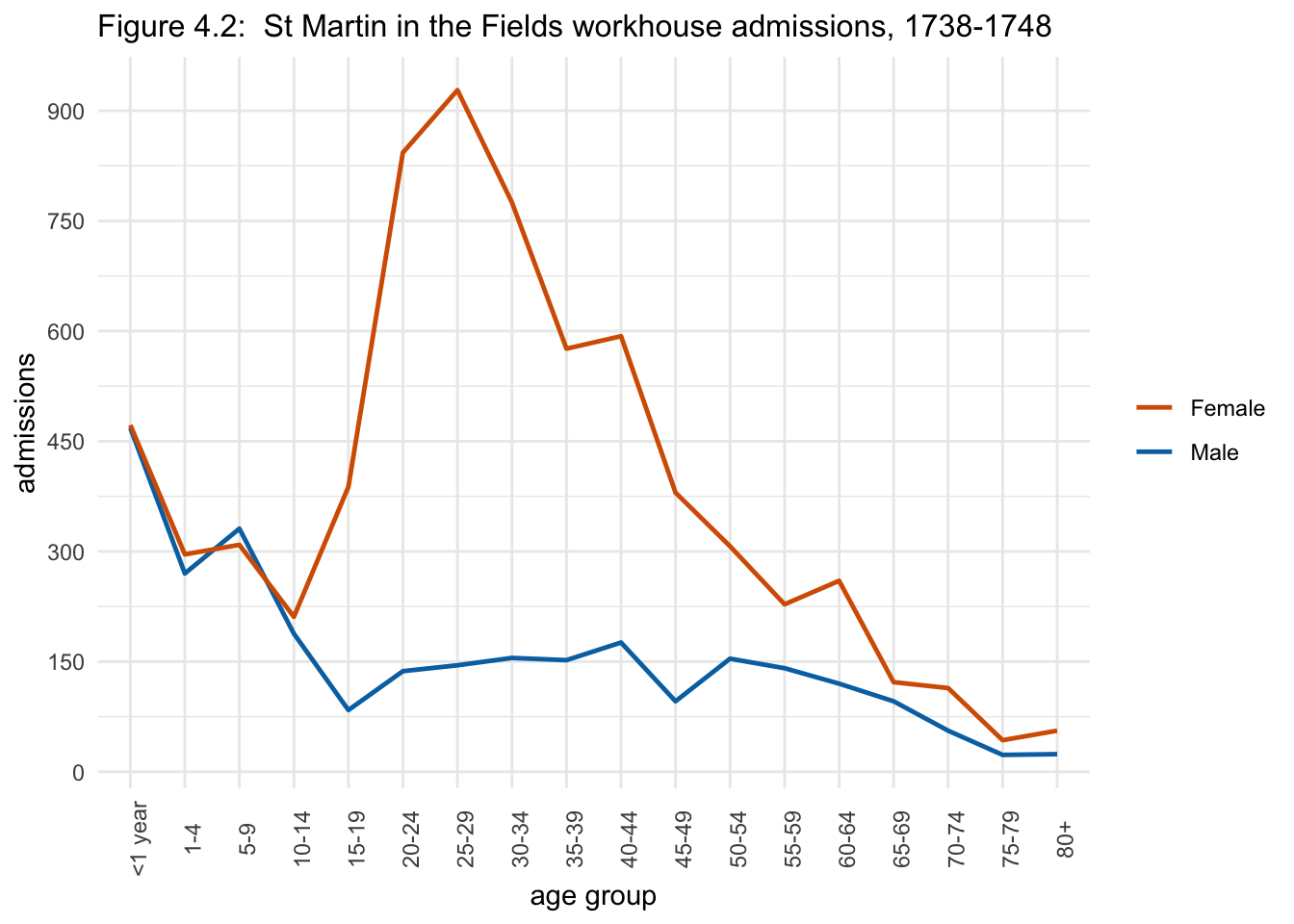

Figure 4.2: St Martin in the Fields workhouse admissions, 1738-1748.

Online dataset: St Martins Workhouse Registers (xlsx)

Pauper Census

c4_scdpc_data <-
  read_xlsx("datasets/St_Clements_Census_of_Pensioners_1745.xlsx", sheet = "Aggregates", range="A3:H20") %>%
  clean_names(case="lower_camel") %>%
  filter(age !="Totals")

c4_scdpc_long <-
  c4_scdpc_data %>%
  select(age, totalGirlsWomen, totalBoysMen) %>%
  gather("k", "v",totalGirlsWomen:totalBoysMen) %>%
  # fix age labels
  mutate(age = fct_recode(age, `80+`= ">80"))  %>%
  mutate(age = str_replace(age, " to ", "-")) %>%
  # fix order of age groups on x axis
  mutate(age = fct_relevel(age, "5-9", after=1L) )


# colours 2 lines
c4_scdpc_long_ggplot <-
c4_scdpc_long %>%
  ggplot(aes(x=age, y=v, colour=k, group=k)) +
  geom_line() +
  scale_y_continuous(breaks = seq(0,40, 5))  +
  scale_colour_manual(values = c("#D55E00", "#0072B2"), 
                      breaks=c("totalGirlsWomen", "totalBoysMen"), 
                      labels=c("Female", "Male")) +
  guides(colour=guide_legend(title=NULL), linetype=guide_legend(title=NULL)) +
  theme(axis.text.x = element_text(angle=90)) +
  labs(x="age group", y="paupers", title = "Figure 4.3: St Clement Danes, Pauper Census, 1745")

c4_scdpc_long_ggplot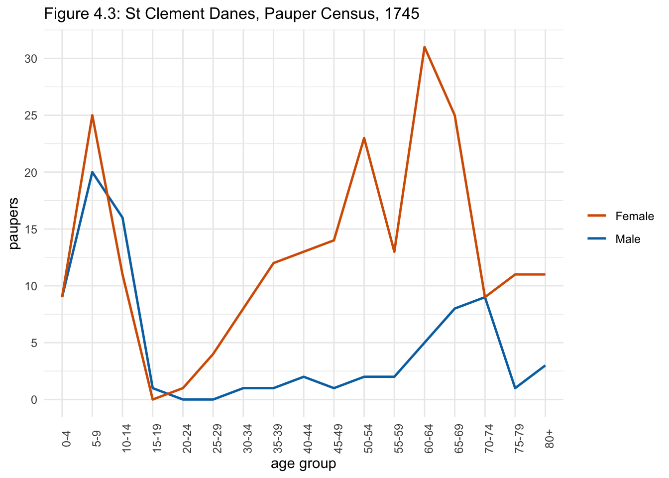

Figure 4.3: St Clement Danes, Pauper Census, 1745.

Online dataset: St Clements Census of Pensioners 1745 (xlsx)

Dropt and Born in the Workhouse

c4_smwhdb <-
  read_xlsx("datasets/St_Martins_Workhouse_Registers.xlsx", sheet = "St Martin's Dropt", skip = 2) %>%
  clean_names(case="lower_camel")

c4_smwhdb_long <-
  c4_smwhdb %>%
  gather("k", "v",droptFoundlingsAndLeft:bornInTheHouse)


# colours 2 lines
c4_smwhdb_long_ggplot <-
c4_smwhdb_long  %>%
  filter(year < 1766) %>%
  ggplot(aes(x=factor(year), y=v, colour=k, group=k)) +
  geom_line() +
  scale_y_continuous(breaks = seq(0,70, 10)) +
  scale_x_discrete(breaks = seq(1725, 1765, 5)) +
  scale_colour_manual(values = c("#D55E00", "#0072B2"), 
                      breaks=c("bornInTheHouse", "droptFoundlingsAndLeft"),  
                      labels=c("Born in \nthe House", "Dropt, \nfoundlings\nand left")) +  
  guides(colour=guide_legend(title=NULL), linetype=guide_legend(title=NULL)) +
  theme(legend.key.height = unit(1.7, "line")) +
  labs(x="year", y="", caption = "data for 1729-1736 do not survive") +
  plot_annotation(title = "Figure 4.4: St Martin in the Fields, Workhouse Registers, 'Dropt' and 'Born in the house'", theme = theme(plot.title = element_text(hjust = 0.5)))

c4_smwhdb_long_ggplot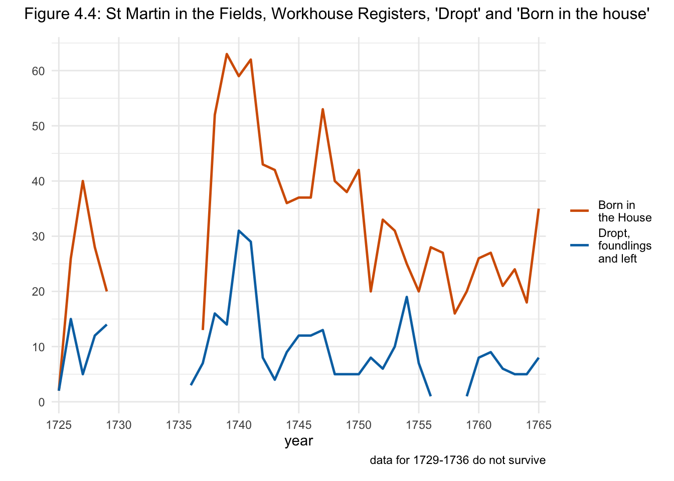

Figure 4.4: St Martin in the Fields, Workhouse Registers, ‘Dropt’ and ‘Born in the house’.

Online dataset: St Martins Workhouse Registers (xlsx)

Legal Counsel

Note that this uses pivot_longer instead of gather. It’s actually pretty cool and I wish I’d started using it earlier!

c4_oblc <-
  read_xlsx("datasets/Legal_Counsel_at_the_Old_Bailey_1715-1800.xlsx", sheet="Legal Counsel at the Old Bailey", skip=2) %>%
  clean_names(case="snake") %>%
  filter(between(year, 1715, 1748)) %>%
  rename(percent_defence_bl=percent_trials_with_defence_counsel_beattie_or_landsman,
         percent_prosecution_bl=percent_trials_with_prosecution_counsel_beattie_or_landsman)


c4_oblc_bl_long <-
  c4_oblc %>%
  select(year, percent_of_trials, percent_defence_bl, percent_prosecution_bl) %>%
  pivot_longer(percent_defence_bl:percent_prosecution_bl, names_to="bl", values_to = "pc_bl")


c4_oblc_bl_long_ggplot <-
c4_oblc_bl_long %>%
  mutate(pl1 = "pc of trials") %>%
  ggplot(aes(x=year)) +
  geom_col(aes(y=pc_bl, fill=bl), position = "dodge") +
  geom_line(aes(y=percent_of_trials, colour=pl1)) +
  scale_colour_manual(values=c("#525252"), breaks=c("pc of trials"), labels=c("% Keyword \n(counsel or \ncross-examined)")) +
  scale_x_continuous(breaks = seq(1715, 1750, 5)) +
  scale_fill_manual(values = c("#56B4E9","#D55E00"), 
                    breaks=c("percent_defence_bl", "percent_prosecution_bl"),  
                    labels=c("% Defence \n(Beattie or \nLandsman)", "% Prosecution \n(Beattie or \nLandsman)")) +
  theme(legend.key.height = unit(2.4, "line"), legend.spacing = unit(0.2, "line")) +
  labs(x="year", y="%", fill=NULL, colour=NULL, title="Figure 4.6: Legal counsel at the Old Bailey, 1715-1748")

c4_oblc_bl_long_ggplot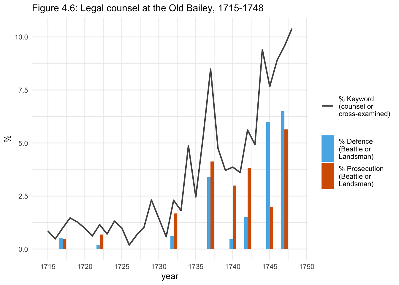

Figure 4.6: Legal counsel at the Old Bailey, 1715-1748

Online dataset: Legal Counsel at the Old Bailey 1715-1800 (xlsx)