Chapter 2: Beggarman, thief: 1690–1713
General notes
The datasets had been released to accompany the original edition of the book and so they’re already cleaner than many spreadsheets. But most of them still needed some reworking before they could be visualised.
I didn’t want to manually edit any of the spreadsheets or make new versions except as a very last resort; the aim is to do all necessary tidying or reformatting within R and leave the original data untouched.
Some of the spreadsheets contain multiple tabs and include data not used in the graphs, so in some cases I had to do a bit of detective work and checking to ensure I was using the right data.
All of the spreadsheets contained titles and other information on the first two lines (minimum) of the sheet, so these lines need to be skipped when reading in the data.
Packages
library(readxl) # read excel spreadsheets
library(janitor) # utilities including clean_names for consistently formatting column names, often a problem with data in spreadsheets
library(lubridate) # date functions
library(scales) # ggplot scales eg %ages
library(patchwork) # extra plot layout options
library(tidyverse) # data wrangling, includes dplyr, tidyr and ggplot

library(knitr)
library(kableExtra)

# ggplot extras ####

theme_set(theme_minimal()) # set preferred ggplot theme
theme_update(plot.title = element_text(size = rel(1.1), hjust = 0)) # adjustments to theme
update_geom_defaults("line", list(size = 0.85))
F2.2: Prosecutions
I’m not going to reproduce all the original b/w graphs, but this is quite a typical example.
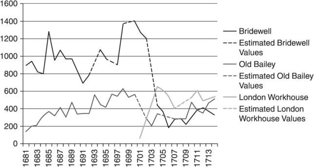
It’s at the more complex end of the visualisations in some respects.
- the data came from multiple spreadsheet tabs which had to be combined
- there was data in “wide” format which needed to be reshaped
- there were gaps in the original sources, filled with estimated values which needed to be differentiated from the known data
Note the use of the clean_names() function from the janitor package. This is invaluable when importing from spreadsheets, which tend to have column names that are not consistently formed and are designed for human rather than machine readers. (R will handle names that contain things like spaces but they have to be enclosed in backticks, which is a bore. I find it easier to convert on importing and then make any nice display labels at the final stage when they’re actually needed.) There are some other great functions in {janitor} that I ought to use more often…
# data from two separate tabs in the spreadsheet
c2_ob <-
  read_xlsx("datasets/Crime_Prosecutions.xlsx", sheet = "Old Bailey", skip = 2) %>%
  clean_names(case="lower_camel")

# and nb this sheet contains data in separate columns for two institutions, Bridewell and the London Workhouse.
c2_bridewell <-
  read_xlsx("datasets/Crime_Prosecutions.xlsx", sheet = "Bridewell", skip = 2) %>%
  clean_names(case="lower_camel")

c2_ob_brd_long <-
# bind_rows() combines the two data frames
# an alternative approach would be to use a full join (on the year column) and then gather
  bind_rows(
    c2_bridewell %>% filter(between(year, 1681,1713)) %>%
    # the Bridewell column was ambiguously named "estimatedValues" so (after checking that it was actually for Bridewell) I renamed it
      select(year, bridewell, londonWorkhouse, bridewellEstimated=estimatedValues, londonWorkhouseEstimated= estimatedLondonWorkhouseValues) %>%
    # gather() to reshape from wide to narrow format
      gather("k", "v", bridewell:londonWorkhouseEstimated)
    ,
    c2_ob %>% filter(between(year, 1681, 1713)) %>%
      select(year, oldBailey= totalCorrected, oldBaileyEstimated = estimatedOldBaileyValues) %>%
      gather("k", "v",oldBailey:oldBaileyEstimated)
  )
# why did I do gathering separately before bind rows? I don't remember, looks a bit daft...
# using "k" and "v" ("key" and "value") as the new column names was just laziness. it's better to use something more meaningful.
What the Bridewell/London Workhouse data looks like before applying gather(). This is classic “wide” format spreadsheet data.
c2_bridewell %>%
  select(year:estimatedLondonWorkhouseValues) %>%
  # knitr::kable() and kableExtra::kable_styling() to make nice tables
  kable() %>%
  kable_styling() %>%
scroll_box(height="400px")| year | bridewell | estimatedValues | londonWorkhouse | estimatedLondonWorkhouseValues |
|---|---|---|---|---|
| 1681 | 896 | NA | NA | NA |
| 1682 | 944 | NA | NA | NA |
| 1683 | 822 | NA | NA | NA |
| 1684 | 804 | NA | NA | NA |
| 1685 | 1279 | NA | NA | NA |
| 1686 | 954 | NA | NA | NA |
| 1687 | 1069 | NA | NA | NA |
| 1688 | 963 | NA | NA | NA |
| 1689 | 973 | NA | NA | NA |
| 1690 | 819 | NA | NA | NA |
| 1691 | 689 | NA | NA | NA |
| 1692 | 781 | 781 | NA | NA |
| 1693 | NA | 927 | NA | NA |
| 1694 | 1072 | 1072 | NA | NA |
| 1695 | 969 | 969 | NA | NA |
| 1696 | NA | 937 | NA | NA |
| 1697 | 904 | 904 | NA | NA |
| 1698 | 1370 | 1370 | NA | NA |
| 1699 | NA | 1388 | NA | NA |
| 1700 | 1406 | 1406 | NA | NA |
| 1701 | 1277 | 1277 | 71 | NA |
| 1702 | 1212 | 1212 | 262 | NA |
| 1703 | NA | 827 | 442 | NA |
| 1704 | 441 | 441 | 653 | NA |
| 1705 | 366 | NA | 611 | NA |
| 1706 | 182 | NA | 540 | NA |
| 1707 | 279 | NA | 405 | 405 |
| 1708 | 290 | NA | NA | 446 |
| 1709 | 225 | NA | NA | 487 |
| 1710 | 299 | NA | 528 | 528 |
| 1711 | 392 | NA | 611 | NA |
| 1712 | 416 | NA | 491 | NA |
| 1713 | 371 | NA | 508 | NA |
| 1714 | 332 | NA | 538 | NA |
| 1715 | NA | NA | NA | NA |
| 1716 | 274 | NA | 363 | NA |
| 1717 | 350 | NA | NA | NA |
| 1718 | 327 | NA | NA | NA |
| 1719 | 288 | NA | NA | NA |
| 1720 | NA | NA | NA | NA |
| 1721 | NA | NA | 683 | NA |
| 1722 | NA | NA | NA | NA |
| 1723 | 293 | NA | 692 | NA |
| 1724 | NA | NA | 750 | NA |
| 1725 | NA | NA | 600 | NA |
| 1726 | NA | NA | 600 | NA |
| 1727 | 317 | NA | 285 | NA |
| 1728 | 257 | NA | 478 | NA |
| 1729 | 179 | NA | 685 | NA |
| 1730 | 331 | NA | 515 | NA |
| 1731 | 572 | NA | 305 | NA |
| 1732 | 673 | NA | 315 | NA |
| 1733 | 612 | NA | 367 | NA |
| 1734 | 325 | NA | 445 | NA |
| 1735 | 325 | NA | 250 | NA |
| 1736 | 465 | 465 | 380 | NA |
| 1737 | NA | 472 | 358 | NA |
| 1738 | 488 | 488 | 358 | NA |
| 1739 | NA | 434 | 358 | NA |
| 1740 | 380 | 380 | 303 | NA |
| 1741 | 372 | 372 | 469 | NA |
| 1742 | NA | 377 | 357 | NA |
| 1743 | 381 | 381 | 265 | NA |
| 1744 | 423 | NA | 207 | NA |
| 1745 | 348 | 348 | 205 | 205 |
| 1746 | NA | 366 | NA | 265 |
| 1747 | NA | 383 | NA | 325 |
| 1748 | 401 | 401 | 384 | 384 |
| 1749 | 378 | NA | 384 | NA |
| 1750 | 322 | 322 | 384 | NA |
| 1751 | NA | 321 | 384 | NA |
| 1752 | NA | 321 | 384 | NA |
| 1753 | 320 | 320 | 384 | NA |
| 1754 | 341 | 341 | 384 | NA |
| 1755 | NA | 333 | NA | NA |
| 1756 | NA | 325 | NA | NA |
| 1757 | NA | 316 | NA | NA |
| 1758 | 308 | 308 | NA | NA |
| 1759 | 245 | NA | NA | NA |
| 1760 | 346 | NA | NA | NA |
| 1761 | 357 | NA | NA | NA |
| 1762 | 579 | NA | NA | NA |
| 1763 | 634 | NA | NA | NA |
| 1764 | 336 | NA | NA | NA |
| 1765 | 392 | NA | NA | NA |
| 1766 | 570 | NA | NA | NA |
| 1767 | 461 | NA | NA | NA |
| 1768 | 569 | NA | NA | NA |
| 1769 | 564 | 564 | NA | NA |
| 1770 | NA | 460 | NA | NA |
| 1771 | 355 | 355 | NA | NA |
| 1772 | 1709 | NA | NA | NA |
| 1773 | 777 | NA | NA | NA |
| 1774 | 808 | NA | NA | NA |
| 1775 | 1084 | NA | NA | NA |
| 1776 | 983 | NA | NA | NA |
| 1777 | 544 | NA | NA | NA |
| 1778 | 1027 | NA | NA | NA |
| 1779 | 681 | NA | NA | NA |
| 1780 | 459 | NA | NA | NA |
| 1781 | 484 | NA | NA | NA |
| 1782 | 659 | NA | NA | NA |
| 1783 | 1597 | NA | NA | NA |
| 1784 | 2956 | NA | NA | NA |
| 1785 | 612 | NA | NA | NA |
| 1786 | 716 | NA | NA | NA |
| 1787 | 865 | NA | NA | NA |
| 1788 | 711 | NA | NA | NA |
| 1789 | NA | NA | NA | NA |
| 1790 | 894 | NA | NA | NA |
| 1791 | 809 | NA | NA | NA |
| 1792 | 1515 | NA | NA | NA |
| 1793 | 1502 | NA | NA | NA |
| 1794 | 1224 | NA | NA | NA |
| 1795 | 1318 | NA | NA | NA |
| 1796 | 1490 | NA | NA | NA |
| 1797 | 1371 | NA | NA | NA |
| 1798 | 1439 | NA | NA | NA |
| 1799 | 1548 | NA | NA | NA |
| 1800 | 1989 | NA | NA | NA |
| 1801 | 1935 | NA | NA | NA |
| 1802 | 1751 | NA | NA | NA |
| 1803 | 1480 | NA | NA | NA |
| 1804 | 1296 | NA | NA | NA |
| 1805 | 1328 | NA | NA | NA |
| 1806 | 1239 | NA | NA | NA |
| 1807 | 1300 | NA | NA | NA |
| 1808 | 1226 | NA | NA | NA |
| 1809 | 553 | NA | NA | NA |
| 1810 | 615 | NA | NA | NA |
And the “wide” Old Bailey data:
c2_ob %>%
  select(year, totalOffences, estimatedOldBaileyValues) %>%
  kable() %>%
  kable_styling() %>%
scroll_box(height="400px")| year | totalOffences | estimatedOldBaileyValues |
|---|---|---|
| 1680 | 127 | NA |
| 1681 | 143 | NA |
| 1682 | 177 | NA |
| 1683 | 217 | NA |
| 1684 | 320 | NA |
| 1685 | 370 | NA |
| 1686 | 319 | NA |
| 1687 | 418 | NA |
| 1688 | 295 | NA |
| 1689 | 299 | NA |
| 1690 | 339 | NA |
| 1691 | 304 | NA |
| 1692 | 259 | NA |
| 1693 | 489 | NA |
| 1694 | 336 | NA |
| 1695 | 366 | NA |
| 1696 | 355 | NA |
| 1697 | 339 | NA |
| 1698 | 394 | NA |
| 1699 | 199 | NA |
| 1700 | 141 | 564.0 |
| 1701 | NA | 432.0 |
| 1702 | 75 | 300.0 |
| 1703 | 78 | NA |
| 1704 | 129 | 344.0 |
| 1705 | NA | 324.3 |
| 1706 | 1 | 304.5 |
| 1707 | 178 | 284.8 |
| 1708 | 176 | NA |
| 1709 | 109 | NA |
| 1710 | 181 | NA |
| 1711 | 189 | NA |
| 1712 | 175 | NA |
| 1713 | 117 | NA |
| 1714 | 320 | NA |
| 1715 | 501 | NA |
| 1716 | 469 | NA |
| 1717 | 451 | NA |
| 1718 | 455 | NA |
| 1719 | 453 | NA |
| 1720 | 449 | NA |
| 1721 | 549 | NA |
| 1722 | 482 | NA |
| 1723 | 475 | NA |
| 1724 | 574 | NA |
| 1725 | 672 | NA |
| 1726 | 595 | NA |
| 1727 | 491 | NA |
| 1728 | 527 | NA |
| 1729 | 607 | NA |
| 1730 | 609 | NA |
| 1731 | 563 | NA |
| 1732 | 526 | NA |
| 1733 | 492 | NA |
| 1734 | 463 | NA |
| 1735 | 596 | NA |
| 1736 | 569 | NA |
| 1737 | 488 | NA |
| 1738 | 397 | NA |
| 1739 | 506 | NA |
| 1740 | 491 | NA |
| 1741 | 539 | NA |
| 1742 | 420 | NA |
| 1743 | 486 | NA |
| 1744 | 440 | NA |
| 1745 | 332 | NA |
| 1746 | 365 | NA |
| 1747 | 369 | NA |
| 1748 | 521 | NA |
| 1749 | 611 | NA |
| 1750 | 569 | NA |
| 1751 | 535 | NA |
| 1752 | 486 | NA |
| 1753 | 503 | NA |
| 1754 | 463 | NA |
| 1755 | 394 | NA |
| 1756 | 386 | NA |
| 1757 | 380 | NA |
| 1758 | 348 | NA |
| 1759 | 326 | NA |
| 1760 | 319 | NA |
| 1761 | 349 | NA |
| 1762 | 315 | NA |
| 1763 | 470 | NA |
| 1764 | 565 | NA |
| 1765 | 484 | NA |
| 1766 | 512 | NA |
| 1767 | 541 | NA |
| 1768 | 548 | NA |
| 1769 | 564 | NA |
| 1770 | 612 | NA |
| 1771 | 710 | NA |
| 1772 | 740 | NA |
| 1773 | 743 | NA |
| 1774 | 735 | NA |
| 1775 | 657 | NA |
| 1776 | 658 | NA |
| 1777 | 658 | NA |
| 1778 | 644 | NA |
| 1779 | 407 | NA |
| 1780 | 565 | NA |
| 1781 | 554 | NA |
| 1782 | 641 | NA |
| 1783 | 922 | NA |
| 1784 | 1104 | NA |
| 1785 | 945 | NA |
| 1786 | 959 | NA |
| 1787 | 872 | NA |
| 1788 | 762 | NA |
| 1789 | 880 | NA |
| 1790 | 751 | NA |
| 1791 | 433 | NA |
| 1792 | 608 | NA |
| 1793 | 726 | NA |
| 1794 | 641 | NA |
| 1795 | 555 | NA |
| 1796 | 659 | NA |
| 1797 | 571 | NA |
| 1798 | 622 | NA |
| 1799 | 604 | NA |
| 1800 | 871 | NA |
What gather() does is to put each of those columns (apart from year) on its own row. After gathering and combining the three sources into one data frame we get:
c2_ob_brd_long %>%
  kable() %>%
  kable_styling() %>%
scroll_box(height="400px")| year | k | v |
|---|---|---|
| 1681 | bridewell | 896.0 |
| 1682 | bridewell | 944.0 |
| 1683 | bridewell | 822.0 |
| 1684 | bridewell | 804.0 |
| 1685 | bridewell | 1279.0 |
| 1686 | bridewell | 954.0 |
| 1687 | bridewell | 1069.0 |
| 1688 | bridewell | 963.0 |
| 1689 | bridewell | 973.0 |
| 1690 | bridewell | 819.0 |
| 1691 | bridewell | 689.0 |
| 1692 | bridewell | 781.0 |
| 1693 | bridewell | NA |
| 1694 | bridewell | 1072.0 |
| 1695 | bridewell | 969.0 |
| 1696 | bridewell | NA |
| 1697 | bridewell | 904.0 |
| 1698 | bridewell | 1370.0 |
| 1699 | bridewell | NA |
| 1700 | bridewell | 1406.0 |
| 1701 | bridewell | 1277.0 |
| 1702 | bridewell | 1212.0 |
| 1703 | bridewell | NA |
| 1704 | bridewell | 441.0 |
| 1705 | bridewell | 366.0 |
| 1706 | bridewell | 182.0 |
| 1707 | bridewell | 279.0 |
| 1708 | bridewell | 290.0 |
| 1709 | bridewell | 225.0 |
| 1710 | bridewell | 299.0 |
| 1711 | bridewell | 392.0 |
| 1712 | bridewell | 416.0 |
| 1713 | bridewell | 371.0 |
| 1681 | londonWorkhouse | NA |
| 1682 | londonWorkhouse | NA |
| 1683 | londonWorkhouse | NA |
| 1684 | londonWorkhouse | NA |
| 1685 | londonWorkhouse | NA |
| 1686 | londonWorkhouse | NA |
| 1687 | londonWorkhouse | NA |
| 1688 | londonWorkhouse | NA |
| 1689 | londonWorkhouse | NA |
| 1690 | londonWorkhouse | NA |
| 1691 | londonWorkhouse | NA |
| 1692 | londonWorkhouse | NA |
| 1693 | londonWorkhouse | NA |
| 1694 | londonWorkhouse | NA |
| 1695 | londonWorkhouse | NA |
| 1696 | londonWorkhouse | NA |
| 1697 | londonWorkhouse | NA |
| 1698 | londonWorkhouse | NA |
| 1699 | londonWorkhouse | NA |
| 1700 | londonWorkhouse | NA |
| 1701 | londonWorkhouse | 71.0 |
| 1702 | londonWorkhouse | 262.0 |
| 1703 | londonWorkhouse | 442.0 |
| 1704 | londonWorkhouse | 653.0 |
| 1705 | londonWorkhouse | 611.0 |
| 1706 | londonWorkhouse | 540.0 |
| 1707 | londonWorkhouse | 405.0 |
| 1708 | londonWorkhouse | NA |
| 1709 | londonWorkhouse | NA |
| 1710 | londonWorkhouse | 528.0 |
| 1711 | londonWorkhouse | 611.0 |
| 1712 | londonWorkhouse | 491.0 |
| 1713 | londonWorkhouse | 508.0 |
| 1681 | bridewellEstimated | NA |
| 1682 | bridewellEstimated | NA |
| 1683 | bridewellEstimated | NA |
| 1684 | bridewellEstimated | NA |
| 1685 | bridewellEstimated | NA |
| 1686 | bridewellEstimated | NA |
| 1687 | bridewellEstimated | NA |
| 1688 | bridewellEstimated | NA |
| 1689 | bridewellEstimated | NA |
| 1690 | bridewellEstimated | NA |
| 1691 | bridewellEstimated | NA |
| 1692 | bridewellEstimated | 781.0 |
| 1693 | bridewellEstimated | 927.0 |
| 1694 | bridewellEstimated | 1072.0 |
| 1695 | bridewellEstimated | 969.0 |
| 1696 | bridewellEstimated | 937.0 |
| 1697 | bridewellEstimated | 904.0 |
| 1698 | bridewellEstimated | 1370.0 |
| 1699 | bridewellEstimated | 1388.0 |
| 1700 | bridewellEstimated | 1406.0 |
| 1701 | bridewellEstimated | 1277.0 |
| 1702 | bridewellEstimated | 1212.0 |
| 1703 | bridewellEstimated | 827.0 |
| 1704 | bridewellEstimated | 441.0 |
| 1705 | bridewellEstimated | NA |
| 1706 | bridewellEstimated | NA |
| 1707 | bridewellEstimated | NA |
| 1708 | bridewellEstimated | NA |
| 1709 | bridewellEstimated | NA |
| 1710 | bridewellEstimated | NA |
| 1711 | bridewellEstimated | NA |
| 1712 | bridewellEstimated | NA |
| 1713 | bridewellEstimated | NA |
| 1681 | londonWorkhouseEstimated | NA |
| 1682 | londonWorkhouseEstimated | NA |
| 1683 | londonWorkhouseEstimated | NA |
| 1684 | londonWorkhouseEstimated | NA |
| 1685 | londonWorkhouseEstimated | NA |
| 1686 | londonWorkhouseEstimated | NA |
| 1687 | londonWorkhouseEstimated | NA |
| 1688 | londonWorkhouseEstimated | NA |
| 1689 | londonWorkhouseEstimated | NA |
| 1690 | londonWorkhouseEstimated | NA |
| 1691 | londonWorkhouseEstimated | NA |
| 1692 | londonWorkhouseEstimated | NA |
| 1693 | londonWorkhouseEstimated | NA |
| 1694 | londonWorkhouseEstimated | NA |
| 1695 | londonWorkhouseEstimated | NA |
| 1696 | londonWorkhouseEstimated | NA |
| 1697 | londonWorkhouseEstimated | NA |
| 1698 | londonWorkhouseEstimated | NA |
| 1699 | londonWorkhouseEstimated | NA |
| 1700 | londonWorkhouseEstimated | NA |
| 1701 | londonWorkhouseEstimated | NA |
| 1702 | londonWorkhouseEstimated | NA |
| 1703 | londonWorkhouseEstimated | NA |
| 1704 | londonWorkhouseEstimated | NA |
| 1705 | londonWorkhouseEstimated | NA |
| 1706 | londonWorkhouseEstimated | NA |
| 1707 | londonWorkhouseEstimated | 405.0 |
| 1708 | londonWorkhouseEstimated | 446.0 |
| 1709 | londonWorkhouseEstimated | 487.0 |
| 1710 | londonWorkhouseEstimated | 528.0 |
| 1711 | londonWorkhouseEstimated | NA |
| 1712 | londonWorkhouseEstimated | NA |
| 1713 | londonWorkhouseEstimated | NA |
| 1681 | oldBailey | 143.0 |
| 1682 | oldBailey | 202.3 |
| 1683 | oldBailey | 217.0 |
| 1684 | oldBailey | 320.0 |
| 1685 | oldBailey | 370.0 |
| 1686 | oldBailey | 319.0 |
| 1687 | oldBailey | 418.0 |
| 1688 | oldBailey | 295.0 |
| 1689 | oldBailey | 478.4 |
| 1690 | oldBailey | 339.0 |
| 1691 | oldBailey | 347.4 |
| 1692 | oldBailey | 345.3 |
| 1693 | oldBailey | 558.9 |
| 1694 | oldBailey | 448.0 |
| 1695 | oldBailey | 418.3 |
| 1696 | oldBailey | 568.0 |
| 1697 | oldBailey | 542.4 |
| 1698 | oldBailey | 630.4 |
| 1699 | oldBailey | 530.7 |
| 1700 | oldBailey | 564.0 |
| 1701 | oldBailey | NA |
| 1702 | oldBailey | 300.0 |
| 1703 | oldBailey | 208.0 |
| 1704 | oldBailey | 344.0 |
| 1705 | oldBailey | NA |
| 1706 | oldBailey | NA |
| 1707 | oldBailey | 284.8 |
| 1708 | oldBailey | 281.6 |
| 1709 | oldBailey | 290.7 |
| 1710 | oldBailey | 482.7 |
| 1711 | oldBailey | 378.0 |
| 1712 | oldBailey | 350.0 |
| 1713 | oldBailey | 468.0 |
| 1681 | oldBaileyEstimated | NA |
| 1682 | oldBaileyEstimated | NA |
| 1683 | oldBaileyEstimated | NA |
| 1684 | oldBaileyEstimated | NA |
| 1685 | oldBaileyEstimated | NA |
| 1686 | oldBaileyEstimated | NA |
| 1687 | oldBaileyEstimated | NA |
| 1688 | oldBaileyEstimated | NA |
| 1689 | oldBaileyEstimated | NA |
| 1690 | oldBaileyEstimated | NA |
| 1691 | oldBaileyEstimated | NA |
| 1692 | oldBaileyEstimated | NA |
| 1693 | oldBaileyEstimated | NA |
| 1694 | oldBaileyEstimated | NA |
| 1695 | oldBaileyEstimated | NA |
| 1696 | oldBaileyEstimated | NA |
| 1697 | oldBaileyEstimated | NA |
| 1698 | oldBaileyEstimated | NA |
| 1699 | oldBaileyEstimated | NA |
| 1700 | oldBaileyEstimated | 564.0 |
| 1701 | oldBaileyEstimated | 432.0 |
| 1702 | oldBaileyEstimated | 300.0 |
| 1703 | oldBaileyEstimated | NA |
| 1704 | oldBaileyEstimated | 344.0 |
| 1705 | oldBaileyEstimated | 324.3 |
| 1706 | oldBaileyEstimated | 304.5 |
| 1707 | oldBaileyEstimated | 284.8 |
| 1708 | oldBaileyEstimated | NA |
| 1709 | oldBaileyEstimated | NA |
| 1710 | oldBaileyEstimated | NA |
| 1711 | oldBaileyEstimated | NA |
| 1712 | oldBaileyEstimated | NA |
| 1713 | oldBaileyEstimated | NA |
What if I’d used a join instead?
c2_brd_ob_join <-
c2_bridewell %>%
  select(year, bridewell, bridewellEstimated=estimatedValues, londonWorkhouse,  londonWorkhouseEstimated=estimatedLondonWorkhouseValues) %>%
  filter(between(year, 1681, 1713)) %>%
  # inner_join is fine here but needs to be used with care because there have to be matching values in *both* tables.
  # sometimes you'd need left_join or full_join, but they can be slower.
  inner_join(
    c2_ob %>%
      select(year, oldBailey= totalCorrected, oldBaileyEstimated = estimatedOldBaileyValues ),
    by="year")

c2_brd_ob_join %>%
  kable() %>%
  kable_styling() %>%
scroll_box(height = "400px")| year | bridewell | bridewellEstimated | londonWorkhouse | londonWorkhouseEstimated | oldBailey | oldBaileyEstimated |
|---|---|---|---|---|---|---|
| 1681 | 896 | NA | NA | NA | 143.0 | NA |
| 1682 | 944 | NA | NA | NA | 202.3 | NA |
| 1683 | 822 | NA | NA | NA | 217.0 | NA |
| 1684 | 804 | NA | NA | NA | 320.0 | NA |
| 1685 | 1279 | NA | NA | NA | 370.0 | NA |
| 1686 | 954 | NA | NA | NA | 319.0 | NA |
| 1687 | 1069 | NA | NA | NA | 418.0 | NA |
| 1688 | 963 | NA | NA | NA | 295.0 | NA |
| 1689 | 973 | NA | NA | NA | 478.4 | NA |
| 1690 | 819 | NA | NA | NA | 339.0 | NA |
| 1691 | 689 | NA | NA | NA | 347.4 | NA |
| 1692 | 781 | 781 | NA | NA | 345.3 | NA |
| 1693 | NA | 927 | NA | NA | 558.9 | NA |
| 1694 | 1072 | 1072 | NA | NA | 448.0 | NA |
| 1695 | 969 | 969 | NA | NA | 418.3 | NA |
| 1696 | NA | 937 | NA | NA | 568.0 | NA |
| 1697 | 904 | 904 | NA | NA | 542.4 | NA |
| 1698 | 1370 | 1370 | NA | NA | 630.4 | NA |
| 1699 | NA | 1388 | NA | NA | 530.7 | NA |
| 1700 | 1406 | 1406 | NA | NA | 564.0 | 564.0 |
| 1701 | 1277 | 1277 | 71 | NA | NA | 432.0 |
| 1702 | 1212 | 1212 | 262 | NA | 300.0 | 300.0 |
| 1703 | NA | 827 | 442 | NA | 208.0 | NA |
| 1704 | 441 | 441 | 653 | NA | 344.0 | 344.0 |
| 1705 | 366 | NA | 611 | NA | NA | 324.3 |
| 1706 | 182 | NA | 540 | NA | NA | 304.5 |
| 1707 | 279 | NA | 405 | 405 | 284.8 | 284.8 |
| 1708 | 290 | NA | NA | 446 | 281.6 | NA |
| 1709 | 225 | NA | NA | 487 | 290.7 | NA |
| 1710 | 299 | NA | 528 | 528 | 482.7 | NA |
| 1711 | 392 | NA | 611 | NA | 378.0 | NA |
| 1712 | 416 | NA | 491 | NA | 350.0 | NA |
| 1713 | 371 | NA | 508 | NA | 468.0 | NA |
And then gather…
c2_brd_ob_join %>%
  gather("k", "v", bridewell:oldBaileyEstimated) %>%
  kable() %>%
  kable_styling() %>%
scroll_box(height = "400px")| year | k | v |
|---|---|---|
| 1681 | bridewell | 896.0 |
| 1682 | bridewell | 944.0 |
| 1683 | bridewell | 822.0 |
| 1684 | bridewell | 804.0 |
| 1685 | bridewell | 1279.0 |
| 1686 | bridewell | 954.0 |
| 1687 | bridewell | 1069.0 |
| 1688 | bridewell | 963.0 |
| 1689 | bridewell | 973.0 |
| 1690 | bridewell | 819.0 |
| 1691 | bridewell | 689.0 |
| 1692 | bridewell | 781.0 |
| 1693 | bridewell | NA |
| 1694 | bridewell | 1072.0 |
| 1695 | bridewell | 969.0 |
| 1696 | bridewell | NA |
| 1697 | bridewell | 904.0 |
| 1698 | bridewell | 1370.0 |
| 1699 | bridewell | NA |
| 1700 | bridewell | 1406.0 |
| 1701 | bridewell | 1277.0 |
| 1702 | bridewell | 1212.0 |
| 1703 | bridewell | NA |
| 1704 | bridewell | 441.0 |
| 1705 | bridewell | 366.0 |
| 1706 | bridewell | 182.0 |
| 1707 | bridewell | 279.0 |
| 1708 | bridewell | 290.0 |
| 1709 | bridewell | 225.0 |
| 1710 | bridewell | 299.0 |
| 1711 | bridewell | 392.0 |
| 1712 | bridewell | 416.0 |
| 1713 | bridewell | 371.0 |
| 1681 | bridewellEstimated | NA |
| 1682 | bridewellEstimated | NA |
| 1683 | bridewellEstimated | NA |
| 1684 | bridewellEstimated | NA |
| 1685 | bridewellEstimated | NA |
| 1686 | bridewellEstimated | NA |
| 1687 | bridewellEstimated | NA |
| 1688 | bridewellEstimated | NA |
| 1689 | bridewellEstimated | NA |
| 1690 | bridewellEstimated | NA |
| 1691 | bridewellEstimated | NA |
| 1692 | bridewellEstimated | 781.0 |
| 1693 | bridewellEstimated | 927.0 |
| 1694 | bridewellEstimated | 1072.0 |
| 1695 | bridewellEstimated | 969.0 |
| 1696 | bridewellEstimated | 937.0 |
| 1697 | bridewellEstimated | 904.0 |
| 1698 | bridewellEstimated | 1370.0 |
| 1699 | bridewellEstimated | 1388.0 |
| 1700 | bridewellEstimated | 1406.0 |
| 1701 | bridewellEstimated | 1277.0 |
| 1702 | bridewellEstimated | 1212.0 |
| 1703 | bridewellEstimated | 827.0 |
| 1704 | bridewellEstimated | 441.0 |
| 1705 | bridewellEstimated | NA |
| 1706 | bridewellEstimated | NA |
| 1707 | bridewellEstimated | NA |
| 1708 | bridewellEstimated | NA |
| 1709 | bridewellEstimated | NA |
| 1710 | bridewellEstimated | NA |
| 1711 | bridewellEstimated | NA |
| 1712 | bridewellEstimated | NA |
| 1713 | bridewellEstimated | NA |
| 1681 | londonWorkhouse | NA |
| 1682 | londonWorkhouse | NA |
| 1683 | londonWorkhouse | NA |
| 1684 | londonWorkhouse | NA |
| 1685 | londonWorkhouse | NA |
| 1686 | londonWorkhouse | NA |
| 1687 | londonWorkhouse | NA |
| 1688 | londonWorkhouse | NA |
| 1689 | londonWorkhouse | NA |
| 1690 | londonWorkhouse | NA |
| 1691 | londonWorkhouse | NA |
| 1692 | londonWorkhouse | NA |
| 1693 | londonWorkhouse | NA |
| 1694 | londonWorkhouse | NA |
| 1695 | londonWorkhouse | NA |
| 1696 | londonWorkhouse | NA |
| 1697 | londonWorkhouse | NA |
| 1698 | londonWorkhouse | NA |
| 1699 | londonWorkhouse | NA |
| 1700 | londonWorkhouse | NA |
| 1701 | londonWorkhouse | 71.0 |
| 1702 | londonWorkhouse | 262.0 |
| 1703 | londonWorkhouse | 442.0 |
| 1704 | londonWorkhouse | 653.0 |
| 1705 | londonWorkhouse | 611.0 |
| 1706 | londonWorkhouse | 540.0 |
| 1707 | londonWorkhouse | 405.0 |
| 1708 | londonWorkhouse | NA |
| 1709 | londonWorkhouse | NA |
| 1710 | londonWorkhouse | 528.0 |
| 1711 | londonWorkhouse | 611.0 |
| 1712 | londonWorkhouse | 491.0 |
| 1713 | londonWorkhouse | 508.0 |
| 1681 | londonWorkhouseEstimated | NA |
| 1682 | londonWorkhouseEstimated | NA |
| 1683 | londonWorkhouseEstimated | NA |
| 1684 | londonWorkhouseEstimated | NA |
| 1685 | londonWorkhouseEstimated | NA |
| 1686 | londonWorkhouseEstimated | NA |
| 1687 | londonWorkhouseEstimated | NA |
| 1688 | londonWorkhouseEstimated | NA |
| 1689 | londonWorkhouseEstimated | NA |
| 1690 | londonWorkhouseEstimated | NA |
| 1691 | londonWorkhouseEstimated | NA |
| 1692 | londonWorkhouseEstimated | NA |
| 1693 | londonWorkhouseEstimated | NA |
| 1694 | londonWorkhouseEstimated | NA |
| 1695 | londonWorkhouseEstimated | NA |
| 1696 | londonWorkhouseEstimated | NA |
| 1697 | londonWorkhouseEstimated | NA |
| 1698 | londonWorkhouseEstimated | NA |
| 1699 | londonWorkhouseEstimated | NA |
| 1700 | londonWorkhouseEstimated | NA |
| 1701 | londonWorkhouseEstimated | NA |
| 1702 | londonWorkhouseEstimated | NA |
| 1703 | londonWorkhouseEstimated | NA |
| 1704 | londonWorkhouseEstimated | NA |
| 1705 | londonWorkhouseEstimated | NA |
| 1706 | londonWorkhouseEstimated | NA |
| 1707 | londonWorkhouseEstimated | 405.0 |
| 1708 | londonWorkhouseEstimated | 446.0 |
| 1709 | londonWorkhouseEstimated | 487.0 |
| 1710 | londonWorkhouseEstimated | 528.0 |
| 1711 | londonWorkhouseEstimated | NA |
| 1712 | londonWorkhouseEstimated | NA |
| 1713 | londonWorkhouseEstimated | NA |
| 1681 | oldBailey | 143.0 |
| 1682 | oldBailey | 202.3 |
| 1683 | oldBailey | 217.0 |
| 1684 | oldBailey | 320.0 |
| 1685 | oldBailey | 370.0 |
| 1686 | oldBailey | 319.0 |
| 1687 | oldBailey | 418.0 |
| 1688 | oldBailey | 295.0 |
| 1689 | oldBailey | 478.4 |
| 1690 | oldBailey | 339.0 |
| 1691 | oldBailey | 347.4 |
| 1692 | oldBailey | 345.3 |
| 1693 | oldBailey | 558.9 |
| 1694 | oldBailey | 448.0 |
| 1695 | oldBailey | 418.3 |
| 1696 | oldBailey | 568.0 |
| 1697 | oldBailey | 542.4 |
| 1698 | oldBailey | 630.4 |
| 1699 | oldBailey | 530.7 |
| 1700 | oldBailey | 564.0 |
| 1701 | oldBailey | NA |
| 1702 | oldBailey | 300.0 |
| 1703 | oldBailey | 208.0 |
| 1704 | oldBailey | 344.0 |
| 1705 | oldBailey | NA |
| 1706 | oldBailey | NA |
| 1707 | oldBailey | 284.8 |
| 1708 | oldBailey | 281.6 |
| 1709 | oldBailey | 290.7 |
| 1710 | oldBailey | 482.7 |
| 1711 | oldBailey | 378.0 |
| 1712 | oldBailey | 350.0 |
| 1713 | oldBailey | 468.0 |
| 1681 | oldBaileyEstimated | NA |
| 1682 | oldBaileyEstimated | NA |
| 1683 | oldBaileyEstimated | NA |
| 1684 | oldBaileyEstimated | NA |
| 1685 | oldBaileyEstimated | NA |
| 1686 | oldBaileyEstimated | NA |
| 1687 | oldBaileyEstimated | NA |
| 1688 | oldBaileyEstimated | NA |
| 1689 | oldBaileyEstimated | NA |
| 1690 | oldBaileyEstimated | NA |
| 1691 | oldBaileyEstimated | NA |
| 1692 | oldBaileyEstimated | NA |
| 1693 | oldBaileyEstimated | NA |
| 1694 | oldBaileyEstimated | NA |
| 1695 | oldBaileyEstimated | NA |
| 1696 | oldBaileyEstimated | NA |
| 1697 | oldBaileyEstimated | NA |
| 1698 | oldBaileyEstimated | NA |
| 1699 | oldBaileyEstimated | NA |
| 1700 | oldBaileyEstimated | 564.0 |
| 1701 | oldBaileyEstimated | 432.0 |
| 1702 | oldBaileyEstimated | 300.0 |
| 1703 | oldBaileyEstimated | NA |
| 1704 | oldBaileyEstimated | 344.0 |
| 1705 | oldBaileyEstimated | 324.3 |
| 1706 | oldBaileyEstimated | 304.5 |
| 1707 | oldBaileyEstimated | 284.8 |
| 1708 | oldBaileyEstimated | NA |
| 1709 | oldBaileyEstimated | NA |
| 1710 | oldBaileyEstimated | NA |
| 1711 | oldBaileyEstimated | NA |
| 1712 | oldBaileyEstimated | NA |
| 1713 | oldBaileyEstimated | NA |
(In R, there are nearly always at least two ways to do the same thing…)
Once the data is in the right shape the ggplot code for a line graph is straightforward, but there are some aesthetic additions:
- use of “linetype” to style the estimated values
- by default ggplot orders legend labels alphabetically so I need to manually re-order
- make nicer display labels (and tweak the legend margins slightly)
- set x and y axis labels
- manual scales give fine grained control over line colours and styling
- the title is unusually long, so it’s split into title and subtitle
# set order of variables in legends
c2_fig2_brk <-
  c("bridewell", "bridewellEstimated", "oldBailey", "oldBaileyEstimated", "londonWorkhouse", "londonWorkhouseEstimated")

# set nice labels
c2_fig2_labels <-
  c("Bridewell", "Estimated\nBridewell", "Old Bailey", "Estimated\nOld Bailey", "London\nWorkhouse", "Est. London\nWorkhouse")


c2_ob_brd_long_ggplot <-
c2_ob_brd_long %>%
  # your aes() stuff can go inside either ggplot() or geom_line()
  # nb linetype for line styling
  ggplot(aes(x=factor(year), y=v, colour=k, group=k, linetype=k)) +
  geom_line() +

  # finesse axis labels
  scale_y_continuous(breaks = seq(0,1600,200), limits = c(0,1600)) +
  scale_x_discrete(breaks = seq(1681, 1714, 2)) +

  # manually control assignment of line colours and add the labels configuration set up earlier
  scale_colour_manual(
    values= c("#D55E00", "#D55E00", "#E69F00", "#E69F00", "#0072B2", "#0072B2"),
    breaks=c2_fig2_brk,
    labels= c2_fig2_labels) +

  # and ditto the linetypes
  # (not at all sure why I gave each series different styling for the estimated values)
  scale_linetype_manual(
    values = c("solid", "dashed", "solid", "dotted", "solid", "dotdash"),
    breaks=c2_fig2_brk,
    labels= c2_fig2_labels) +

  # hide unwanted legend title
  guides(colour=guide_legend(title=NULL),
         linetype=guide_legend(title=NULL)) +

  # some nitpicky fiddling with legend margins
  theme(legend.text = element_text(margin = margin(t = 0.1, b=0.1, unit = "cm")) ) +

  # and add nice display labels
  labs(x="year", y="number",
       title="Figure 2.2: Prosecutions and commitments, 1681–1714",
       subtitle="The Old Bailey, Bridewell and London Workhouse")
c2_ob_brd_long_ggplot ## Warning: Removed 94 row(s)
## containing missing values
## (geom_path).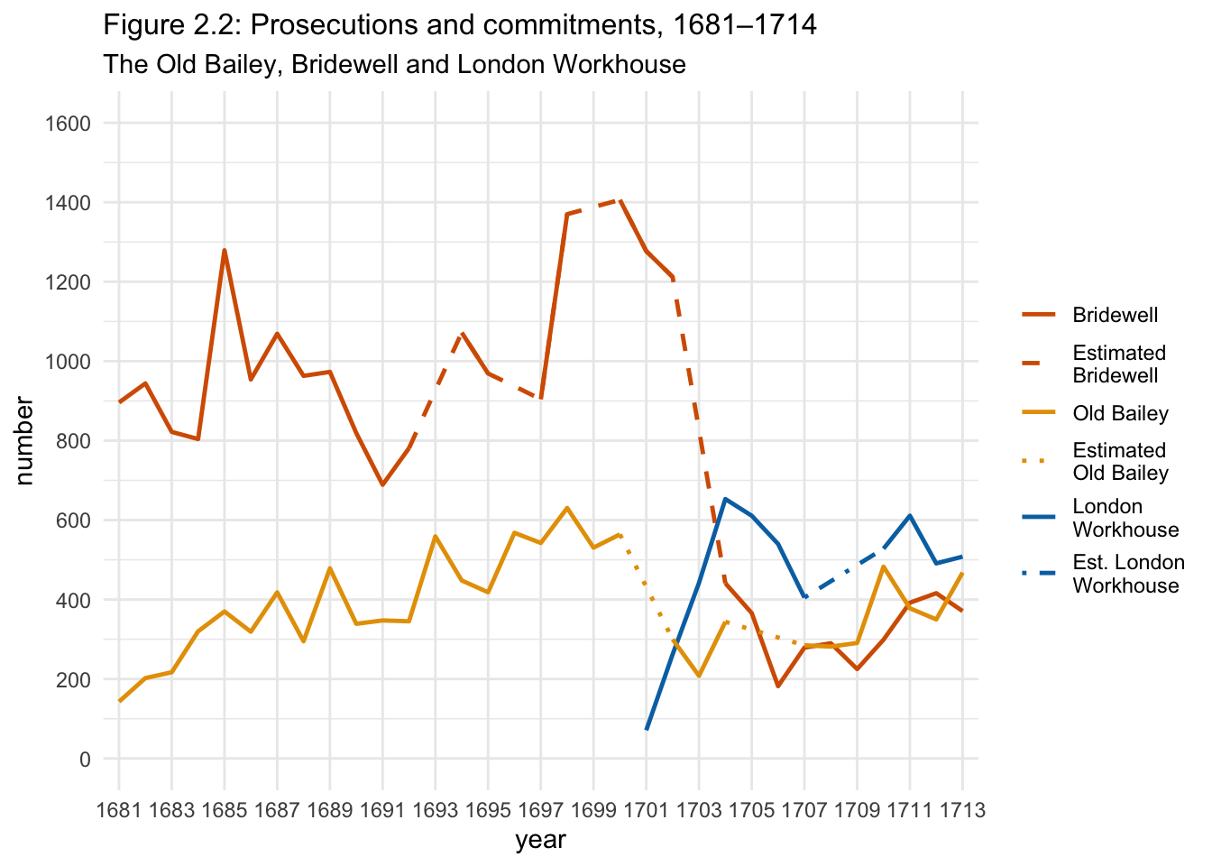
Figure 2.2: Prosecutions and commitments, 1681–1714: The Old Bailey, Bridewell and London Workhouse
A reminder of what the original looked like.
Online dataset: Crime Prosecutions (xlsx)
F2.3: Vice Offences
This one is simpler.
c2_lm_books <-
  read_xlsx("datasets/LM_Waiting_and_Charge_Books_1686-1733.xlsx", sheet = "Data", skip = 2)  %>%
  clean_names(case="lower_camel")

c2_lm_books_ggplot <-
c2_lm_books %>%
  # no idea why I decided to filter the years like this instead of using between()
  filter(year %in% c(1686, 1687, 1688, 1689, 1690, 1691, 1692, 1693, 1694) ) %>%
  gather("type", "counts", prostitution:total) %>%
  ggplot(aes(x=year, y= counts, group=type, colour=type)) +
  geom_line() +
  # didn't bother to create the breaks and labels beforehand this time
  scale_colour_manual(
    breaks=c("total", "drunkenness", "prostitution", "sabbathBreaking", "swearing"),
    labels=c("Total", "Drunkenness", "Prostitution", "Sabbath\nBreaking", "Swearing"),
    values = c("#D55E00", "#E69F00", "#0072B2", "#F0E442", "#CC79A7"))+
  guides(colour=guide_legend(title=NULL))  +
  labs(x="year", y="number of offences") +

  # using patchwork::plot_annotation() a bit fudgily here for cosmetic reasons:
  # this was a particularly long plot title and it creates more space to fit it in
  plot_annotation(title="Figure 2.3: Vice offences recorded in Lord Mayor's waiting and charge books, 1686-1694", theme = theme(plot.title = element_text(hjust = 0.5)))
c2_lm_books_ggplot 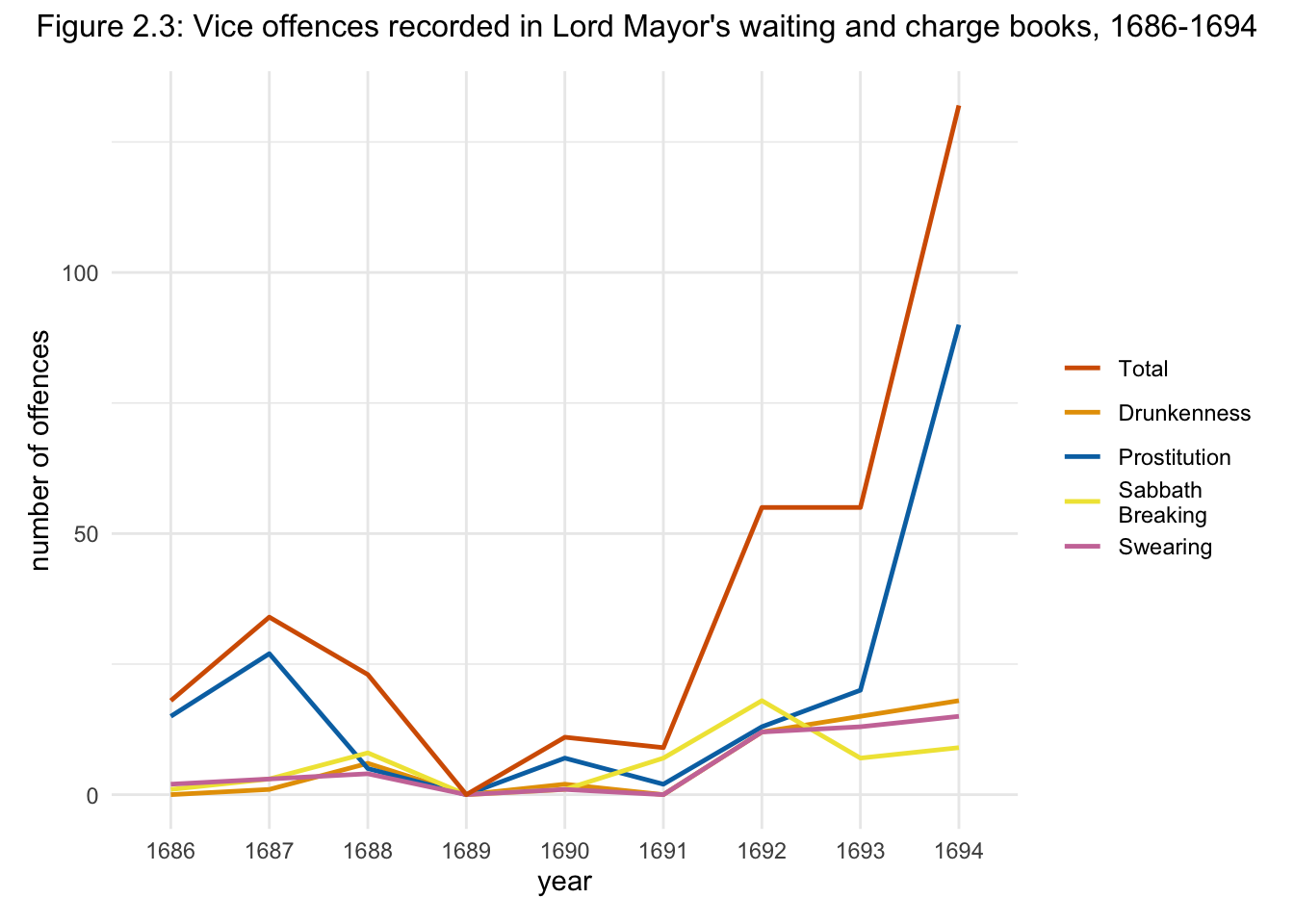
Figure 2.3: Vice offences recorded in Lord Mayor’s waiting and charge books, 1686-1694
Online dataset: LM Waiting and Charge Books 1686-1733 (xlsx)