Chapter 7: The state in chaos: 1776–1789

link to chapter 7

Packages

library(readxl)
library(janitor)
library(lubridate)
library(scales)
library(patchwork)

library(tidyverse)

# ggplot_extras ####

theme_set(theme_minimal()) # set preferred ggplot theme 
theme_update(plot.title = element_text(size = rel(1.1), hjust = 0)) # adjustments to theme
update_geom_defaults("line", list(size = 0.85))

Escapes

(OK, this one is not perhaps best practice. But I think it works ok.)

c7_escapees <-
  read_excel("datasets/Escapes_1776-1786.xlsx", sheet = "Total Escapees", skip = 1) %>%
  clean_names(case="snake")


c7_escapees_ggplot <-
c7_escapees %>%
  select(year, escapees_including_attempts, gordon_riots) %>%
  # make gordon_riots + escapees add up to 250 so that bar goes up to the top of the plot
  mutate(gordon_riots = gordon_riots - 1358) %>% 
  pivot_longer(escapees_including_attempts:gordon_riots, names_to="esc", values_to = "v") %>%
  filter(!is.na(v)) %>%
  mutate(esc = fct_relevel(esc, "gordon_riots", "escapees_including_attempts")) %>%
  ggplot(aes(x=factor(year), y=v, fill=esc)) +
  geom_col() +
  # add text to the gordon riots bars to show that it goes off the top of the chart
  annotate("text", x = 5, y = 230, label = "The Gordon Riots, June 1780\nc.1600 escapes") +
  scale_y_continuous(limits = c(0,250), breaks=seq(0, 200, 50), expand = c(0,0.2)) +
  scale_fill_manual(labels=c("Gordon Riots", "Escapees\nincluding\nattempts"),
                    values=c("#E69F00", "#D55E00")) +
  theme(legend.key.height = unit(1.8, "line")) +
  labs(x="year", y="Escapees", fill=NULL)  +
  plot_annotation(title = "Figure 7.2: Escapees (attempted and actual) from prisons, hulks and transports, 1776-1786", theme = theme(plot.title = element_text(hjust = 0.5)))

c7_escapees_ggplot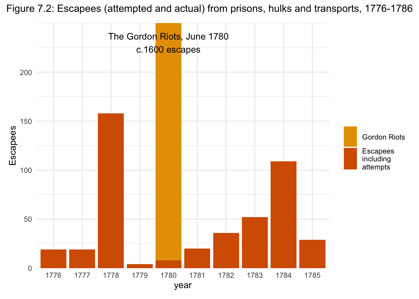

Figure 7.2: Escapees (attempted and actual) from prisons, hulks and transports, 1776-1786.

Online dataset: Escapes 1776-1786 (xlsx)

Prosecutions

c7_ob <-
  read_xlsx("datasets/Crime_Prosecutions.xlsx", sheet = "Old Bailey", skip = 2) %>%
  clean_names(case="snake")

c7_bridewell <-
  read_xlsx("datasets/Crime_Prosecutions.xlsx", sheet = "Bridewell", skip = 2) %>%
  clean_names(case="snake")

c7_ob_brd <-
  bind_rows(
    c7_bridewell %>%
      filter(between(year, 1775,1789)) %>%
      select(year, total= bridewell) %>%
      mutate(src="Bridewell")
    ,
    c7_ob %>% filter(between(year, 1775, 1789)) %>%
      select(year, total= total_offences) %>%
      mutate(src="Old Bailey")
  )


c7_ob_brd_ggplot <-
c7_ob_brd %>%
  mutate(src = fct_relevel(src, "Old Bailey", "Bridewell")) %>%
  ggplot(aes(x=year, y=total, colour=src)) +
  geom_line() +
  facet_wrap(~src, ncol = 1, scales="free_y") +
  scale_colour_manual(values=c("#0072B2", "#D55E00")) +
  scale_x_continuous(breaks = seq(1775, 1790, 2)) +
  guides(colour=FALSE) +
  labs(x="year", title="Figure 7.6: Prosecutions and commitments, 1775-1789", colour=NULL)

c7_ob_brd_ggplot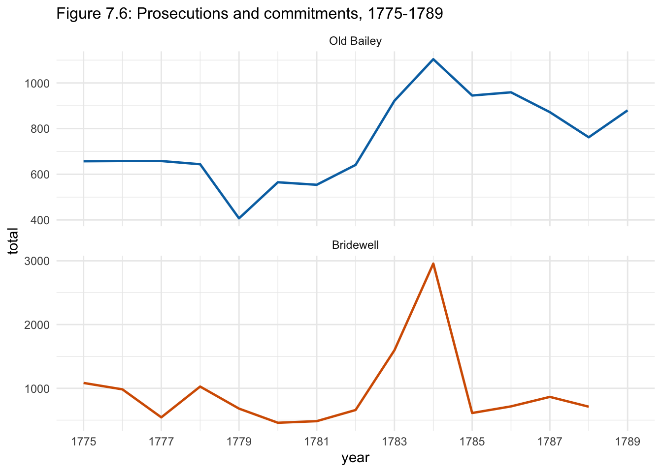

Figure 7.6: Prosecutions and commitments, 1775-1789.

Online dataset: Crime Prosecutions (xlsx)

Old Bailey Legal Counsel

c7_oblc <-
  read_xlsx("datasets/Legal_Counsel_at_the_Old_Bailey_1715-1800.xlsx", sheet="Legal Counsel at the Old Bailey", skip=2) %>%
  clean_names(case="snake") %>%
  filter(between(year, 1770, 1800))  %>%
  rename(percent_defence_bl=percent_trials_with_defence_counsel_beattie_or_landsman, percent_prosecution_bl=percent_trials_with_prosecution_counsel_beattie_or_landsman)


c7_oblc_bl_long <-
  c7_oblc %>%
  select(year, percent_of_trials, percent_defence_bl, percent_prosecution_bl) %>%
  pivot_longer(percent_defence_bl:percent_prosecution_bl, names_to="bl", values_to = "pc_bl")


c7_oblc_bl_long_ggplot <-
c7_oblc_bl_long %>%
  mutate(pl1 = "pc of trials") %>%
  ggplot(aes(x=year)) +
  geom_col(aes(y=pc_bl, fill=bl), position = "dodge") +
  geom_line(aes(y=percent_of_trials, colour=pl1)) +
  scale_x_continuous(breaks = seq(1770, 1800, 5)) +
  scale_colour_manual(values=c("black"), breaks=c("pc of trials"), 
                      labels=c("% Keyword \n(counsel or \ncross-examined)")) +
  scale_fill_manual(breaks=c("percent_defence_bl", "percent_prosecution_bl"),  
                    labels=c("% Defence \n(Beattie or \nLandsman)", "% Prosecution \n(Beattie or \nLandsman)"), 
                    values=c("#56B4E9", "#D55E00")) +
  theme(legend.text = element_text(margin = margin(t = 0.2, b=0.2, unit = "cm")), legend.spacing = unit(0.1, "line") )  +
  labs(fill=NULL, colour=NULL, y="% of trials", title="Figure 7.7: Percentage of Old Bailey trials with legal counsel, 1770-1800", caption="as reported in the Proceedings")

c7_oblc_bl_long_ggplot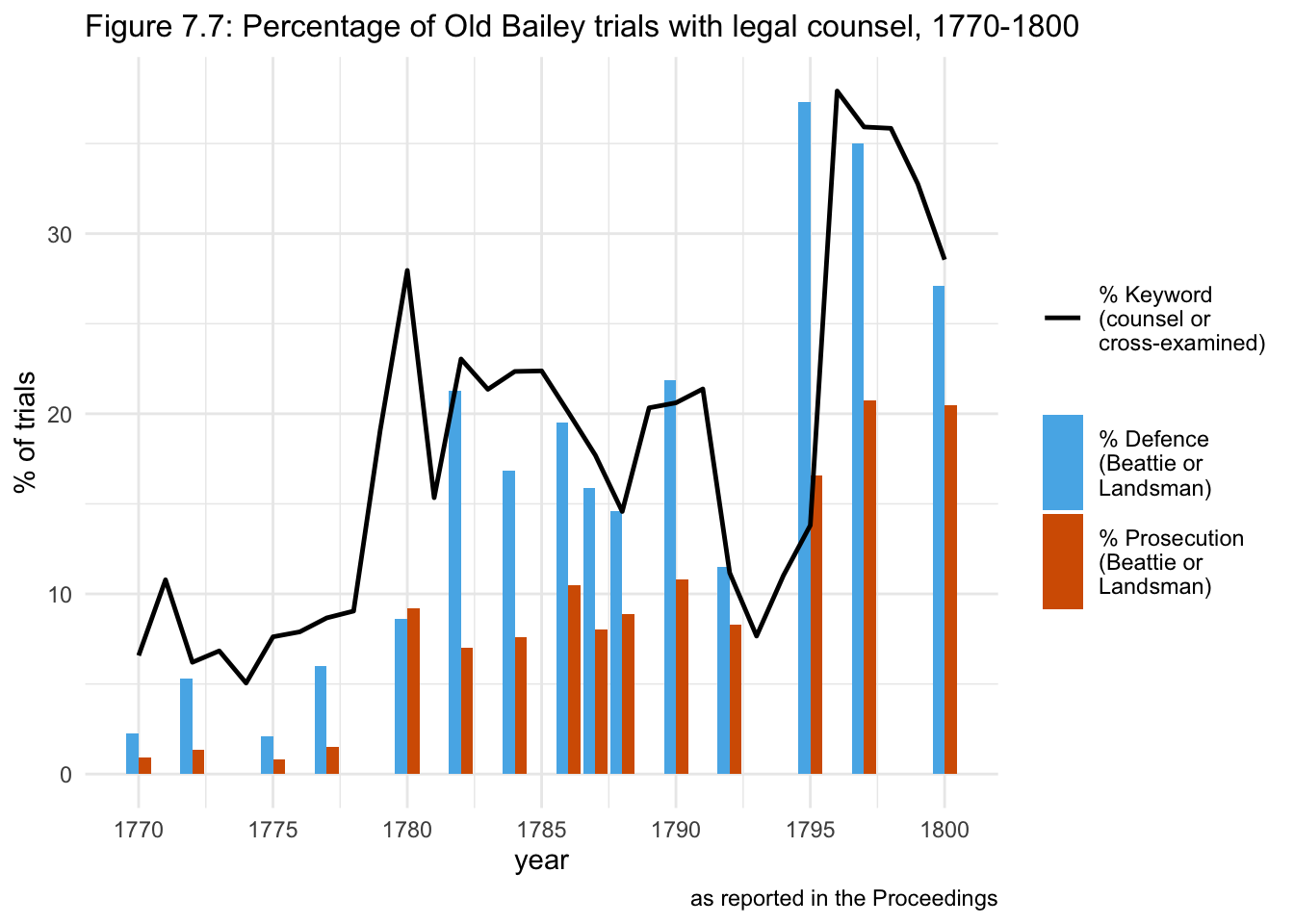

Figure 7.7: Percentage of Old Bailey trials with legal counsel, 1770-1800, as reported in the Proceedings.

Online dataset: Legal Counsel at the Old Bailey 1715-1800 (xlsx)

Old Bailey Sentences

c7_punob <-
  read_xlsx("datasets/Punishment_Statistics_1690-1800.xlsx", sheet = "Old Bailey Punishments", skip=2) %>%
  clean_names(case="lower_camel") %>%
  filter(x1 !="Total") %>%
  rename(year=x1) %>% mutate(year = as.double(year))

## New names:
## * `` -> ...1
## * `%` -> `%...4`
## * `%` -> `%...6`
## * `%` -> `%...8`
## * `%` -> `%...10`
## * ...

pun_long_1770 <-
  c7_punob %>%
  filter(between(year, 1770, 1790)) %>%
  select(year, total, corporal, death, transportation, imprisonment, branding, miscNoPun= miscellaneousAndNoPunishment) %>%
  gather("k", "v",corporal:miscNoPun) %>%
  mutate(pc = v/total*100)


c7_pun_long_1770_ggplot <-
pun_long_1770  %>%
  ggplot(aes(x=factor(year), y=pc, colour=k, group=k)) +
  geom_line() +
  scale_y_continuous(breaks = seq(0,80,10), limits = c(0,80)) +
  scale_colour_manual(breaks=c("transportation", "imprisonment", "corporal", "death", "branding", "miscNoPun"),
                      labels=c("Transportation", "Imprisonment", "Corporal", "Death", "Branding", "Miscellaneous/\nNo Punishment"),
                      values=c("#0072B2", "#E69F00", "#D55E00", "#56B4E9", "#F0E442", "#CC79A7") ) +
  scale_x_discrete(breaks = seq(1770, 1790, 2)) +
  guides(colour=guide_legend(title=NULL), linetype=guide_legend(title=NULL)) +
  labs(x="year", y="% of sentences", title = "Figure 7.8 Old Bailey punishment sentences, 1770-1790")

# order: transportation, imprisonment, corporal, death, branding, miscellaneous and no punishment

c7_pun_long_1770_ggplot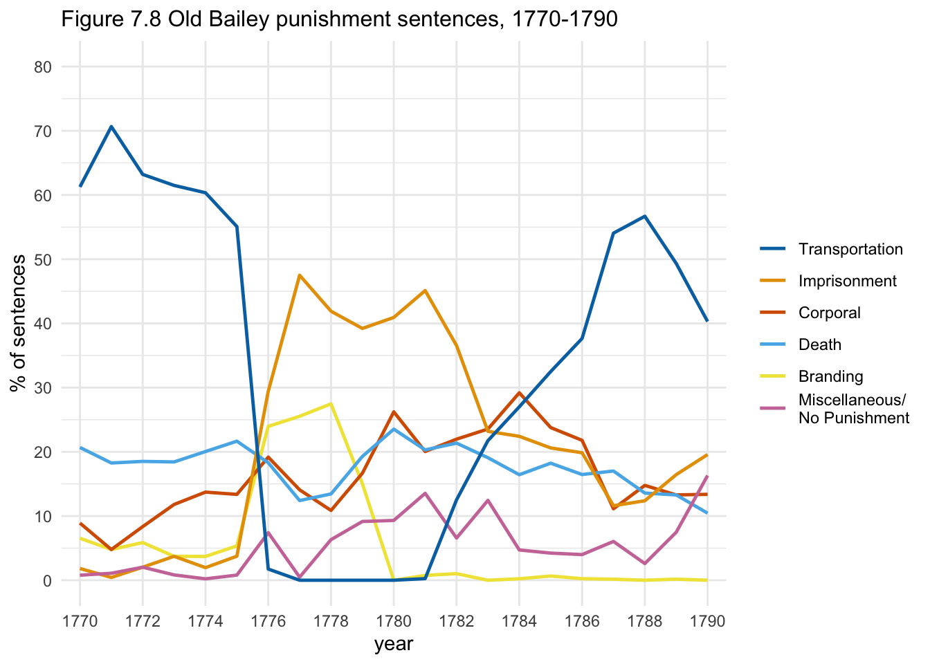

Figure 7.8 Old Bailey punishment sentences, 1770-1790.

Online dataset: Punishment Statistics 1690-1800 (xlsx)

Death Sentences and Executions

Combine two types of plot in one (using {patchwork}).

ob_death_executions_1775 <-
  read_excel("datasets/Death_Sentences_and_Executions_1749-1806.xlsx", skip=2, sheet="Data") %>%
  clean_names(case="snake") %>%
  filter(between(year, 1775, 1790)) %>%
  select(year, condemned, executed, percent_executed)


c7_ob_death_executions_1775_ggplot <-
ob_death_executions_1775 %>%
  mutate(not_executed = condemned-executed) %>%
  select(-percent_executed, -condemned) %>%
  pivot_longer(executed:not_executed, names_to = "condemned", values_to = "v") %>%
  ggplot(aes(x=year, y=v, fill=condemned)) +
  geom_col()+
  scale_x_continuous(breaks=seq(1776, 1790, 2), expand = c(0,0))  +
  scale_y_continuous(breaks=seq(0, 180, 30)) +
  scale_fill_manual(values=c("#D55E00", "#E69F00"), 
                    label = c("executed", "not executed")) +
  labs(fill=NULL, y="sentences") +
  
ob_death_executions_1775 %>%
  ggplot(aes(year, percent_executed)) +
  geom_line(colour="#0072B2")+
  scale_y_continuous(limits = c(0,100)) +
  scale_x_continuous(breaks=seq(1776, 1790, 2), expand = c(0,0)) +
  labs(y="% executed", colour=NULL, linetype=NULL) +
  
plot_annotation(title = "Figure 7.9: Old Bailey death sentences and executions, 1775-1790") +
plot_layout(ncol=1, heights=c(5,3))

c7_ob_death_executions_1775_ggplot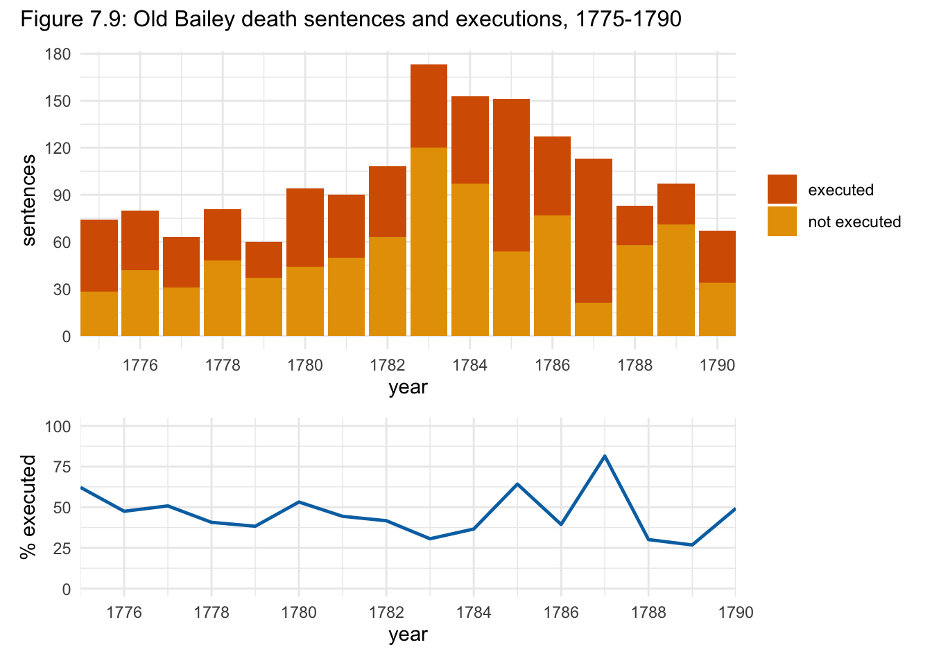

Figure 7.9: Old Bailey death sentences and executions, 1775-1790.

Online dataset: Death Sentences and Executions 1749-1806 (xlsx)

Whipping Punishments

c7_whippings_data <-
  read_excel("datasets/London_Whipping_Punishments_1770-1799.xlsx", skip=2, sheet="London Whipping Punishments") %>%
  clean_names(case="snake") %>%
  rename(year=x1)

## New names:
## * `` -> ...1

c7_whippings_data_ggplot <-
c7_whippings_data %>%
  mutate(private = all_whippings-public) %>%
  select(-percent_public, -all_whippings) %>%
  pivot_longer(public:private, names_to = "whippings", values_to = "v") %>%
  mutate(whippings = fct_relevel(whippings, "public", "private")) %>%
  ggplot(aes(x=year, y=v, fill=whippings)) +
  geom_col() +
  scale_x_continuous(breaks=seq(1770, 1799, 2), expand = c(0,0))  +
  scale_fill_manual( values=c("#D55E00", "#E69F00") ) +
  labs(fill=NULL, y="whippings") +
  
  c7_whippings_data %>%
  ggplot(aes(year, percent_public)) +
  geom_line()+
  scale_y_continuous(limits = c(0,75)) +
  scale_x_continuous(breaks=seq(1770, 1799, 2), expand = c(0,0))  +
  labs(y="% public") +
  
  plot_annotation(title = "Figure 7.10: London whipping punishments, 1770-1799") +
  plot_layout(ncol=1, heights=c(4,3))

c7_whippings_data_ggplot

## Warning: Removed 2 rows containing
## missing values
## (position_stack).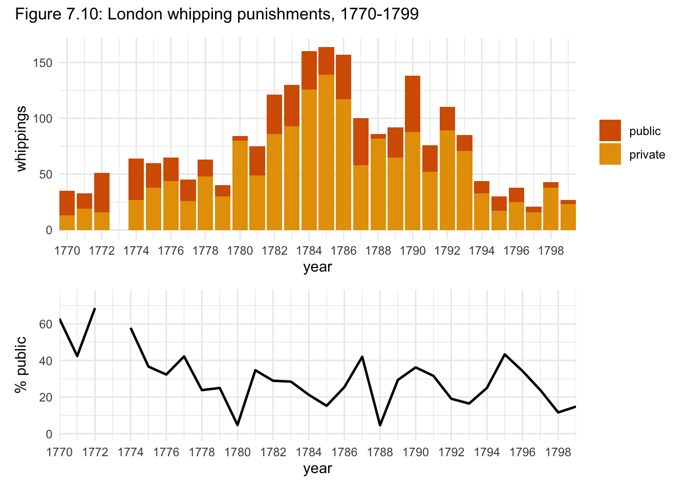

Figure 7.10: London whipping punishments, 1770-1799.

Online dataset: London Whipping Punishments 1770-1799 (xlsx)

Poor Law Expenditure

c7_scd_poor_spend <-
  read_excel("datasets/St_Clement_Danes_Poor_Law_Expenditure_1706-1803.xlsx", skip=2, sheet = "St Clement") %>%
  clean_names(case="snake") %>%
  filter(between(year, 1750, 1803)) %>%
  # zoo::rollmean() for moving average
  mutate(movinga = zoo::rollmean(monthly_total_poor_law_accounts, k=5, fill=NA))



c7_scd_poor_spend_long2 <-
  bind_rows(
    c7_scd_poor_spend %>%
      select(year, stcd_parl= st_clements_dane_parliamentary_returns) %>%
      mutate(recs="parl") ,
    c7_scd_poor_spend %>%
      select(year, stcd_pr= monthly_total_poor_law_accounts, movinga) %>%
      pivot_longer(stcd_pr:movinga, names_to = "stcd_parish", values_to = "v") %>%
      mutate(recs = "parish_recs")
  )



c7_scd_poor_spend_long2_ggplot <-
c7_scd_poor_spend_long2 %>%
  ggplot(aes(x=year)) +
  geom_col(aes(y=stcd_parl, fill=recs)) +
  geom_line(aes(y=v, colour=stcd_parish, linetype=stcd_parish)) +
  scale_x_continuous(breaks=seq(1750,1804,4))  +
  scale_fill_manual(values = c("#D55E00"), labels=c("Parliamentary\nreturns"))  +
  scale_colour_manual(na.translate=FALSE,  # na.translate gets rid of NA in legend
                      breaks=c("stcd_pr", "movinga"),
                      labels=c("Parish\naccounts", "Parish accounts\n(5 yr moving \naverage)"),
                      values=c("#000000","#525252")) +  
  scale_linetype_manual(na.translate=FALSE,
                        breaks=c("stcd_pr", "movinga"),
                        labels=c("Parish\naccounts", "Parish accounts\n(5 yr moving \naverage)"),
                        values=c("solid", "dotted")
  ) +
  theme(legend.key.height = unit(1.7, "line"), legend.spacing = unit(0.2, "line") ) +
  guides(colour=guide_legend(title=NULL), fill=guide_legend(title=NULL), linetype=guide_legend(title=NULL)) +
  labs(y="£", title= "Figure 7.12: St Clement Danes, poor law expenditure, 1750--1803")

c7_scd_poor_spend_long2_ggplot

## Warning: Removed 154 rows containing
## missing values
## (position_stack).

## Warning: Removed 64 row(s)
## containing missing values
## (geom_path).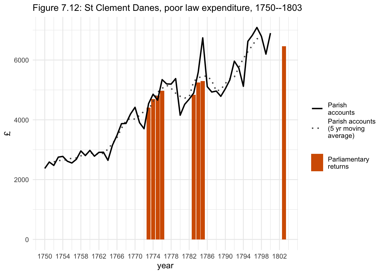

Figure 7.12: St Clement Danes, poor law expenditure, 1750–1803.

Online dataset: St Clement Danes Poor Law Expenditure 1706-1803 (xlsx)

Vagrant Expenditure

c7_col_vagrant_expend_data <-
  read_excel("datasets/City_of_London_Vagrant_Expenditure_1738-1792.xlsx", skip=2, sheet = "Vagrant Expenditure") %>%
  clean_names(case="snake") %>%
  filter(between(year, 1776, 1790))


c7_col_vagrant_expend_data_ggplot <-
c7_col_vagrant_expend_data  %>%
  select(year, expenditure= total_expenditure_to_the_nearest) %>%
  ggplot(aes(x=year, y=expenditure)) +
  geom_line() +
  scale_x_continuous(breaks = seq(1776,1790,2)) +
  labs(y="expenditure (£)", title = "Figure 7.13: City of London vagrancy expenditure, 1776-1790")

c7_col_vagrant_expend_data_ggplot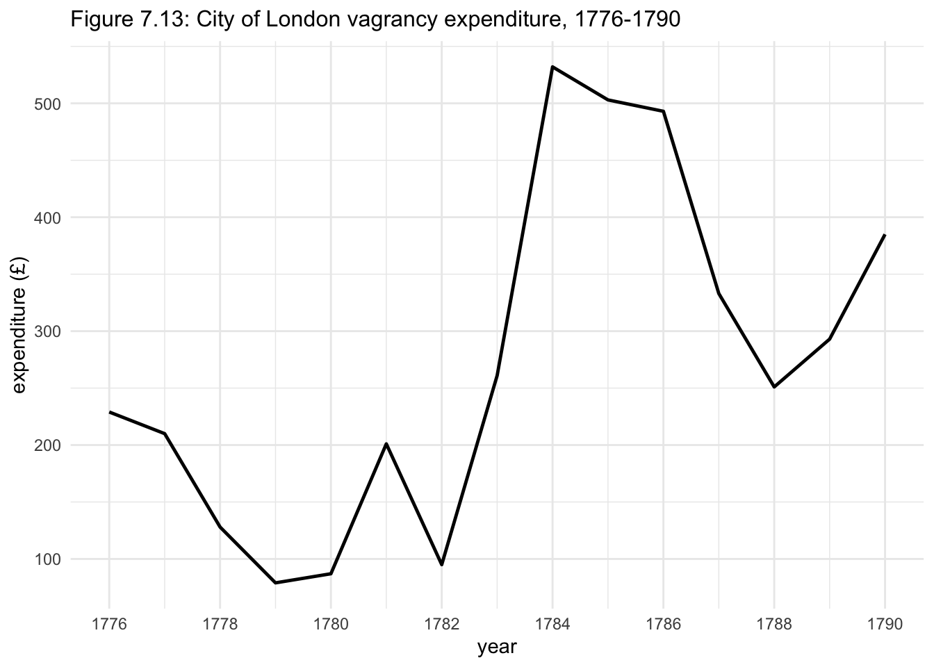

Figure 7.13: City of London vagrancy expenditure, 1776-1790.

Online dataset: City of London Vagrant Expenditure 1738-1792 (xlsx)